Drawing Astrolabes: The Plate Grid
- Ray
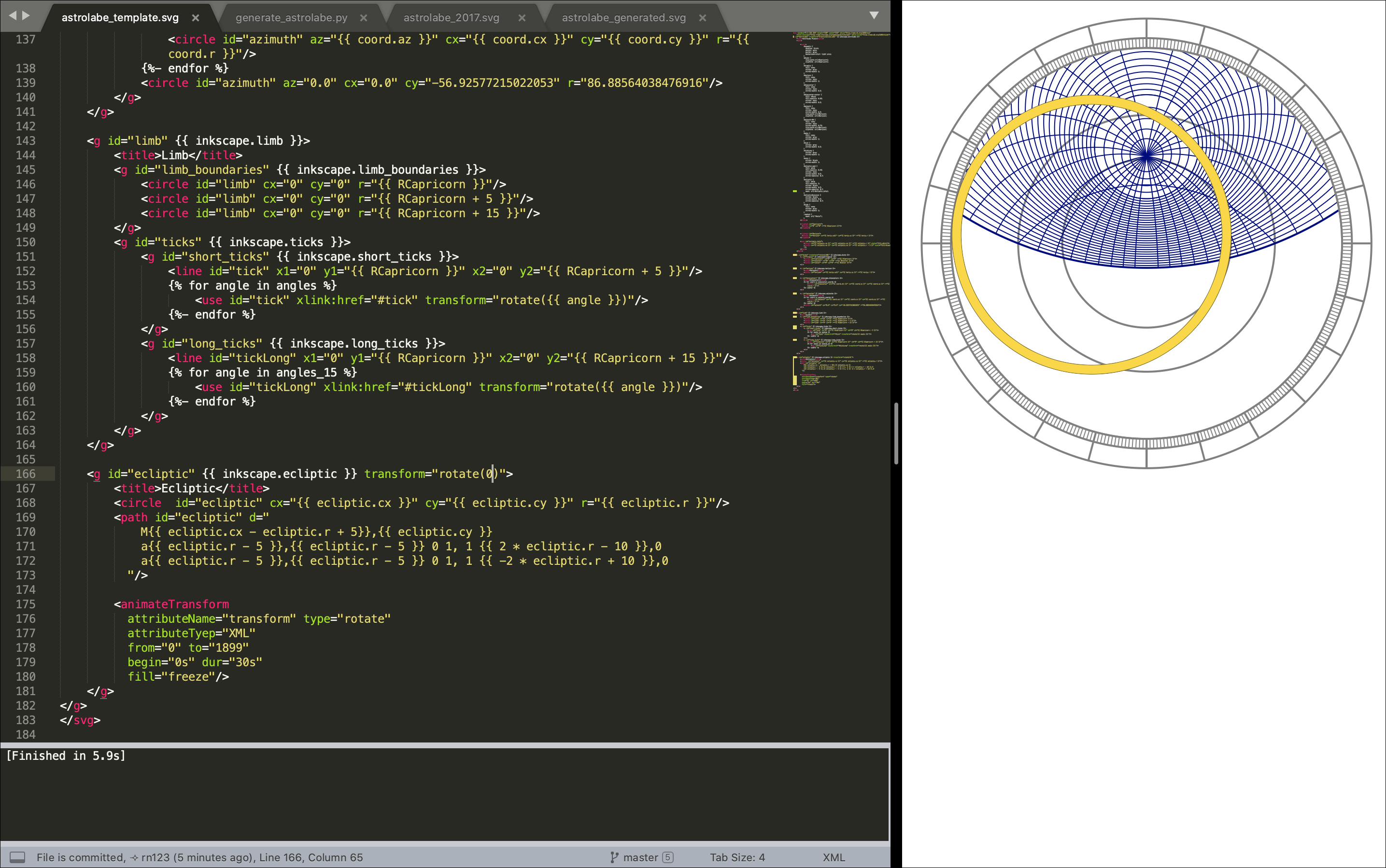
The plate grid of an astrolabe is the stereographic projection of the celestial sphere through the south celestial pole onto the plane of the equator. Quoting Morrison:
The interior of the plate can be thought of as a special kind of graph paper for finding the location of celestial objects in the sky at your location. The main difference between normal graph paper and the graph paper on the plate is the lines on graph paper are normally straight while the astrolabe lines are curve. All of the curves on the astrolabe plate are drawn as arcs of circles.
Ultimately, all that is needed to draw the plate of an astrolabe is to draw a bunch of circles. It all boils down to finding the center and radius of each circle. In order to show only the visible sky above the horizon, the circles are clipped to lie in a given area.
Continuing, here is Morrisons basic description:
The larger circles centered on the plate represent the Earth’s tropics. The largest circle, which defines the outside of the plate, is the Tropic of Capricorn, which is the farthest south the sun ever reaches. The middle circle is the equator and the smaller circle is the sun’s northern limit, the Tropic of Cancer. The circles defining the tropic are the same for all latitudes.
 Not mentioned is the dependency of the plate on the obliquity of the ecliptic – the angle that the plane of the Sun’s path makes with the Earth’s equator. Modern celestial mechanics starts with the identification of the time dependence of the obliquity of the ecliptic. Drawing historically accurate diagrams needs to take into account this time dependency. The story of this discovery and how the obliquity was measured five hundred years ago appears in Heilbron’s book, “The Sun in the Church.”
Morrison continues:
The straight lines drawn as diameters of the largest circle show direction. The vertical diameter goes north and south through your location, representing your meridian. South is at the top and east to the left. The horizontal diameter connects east and west and is the projection of the great circle perpendicular to the meridian. It is normally called the right horizon, the horizon at the equator. It is perhaps easiest to visualize the plate as lying flat on a table with the top pointing south. A star chart is held overhead. You look down on an astrolabe, like a compass.
Morrison’s book has details about the layout of many tools based on stereographic projections. In particular, he does have a chapter on generating star finders. Continuing with the description:
The plate is used to find the positions of celestial objects in the sky as seen by an observer at a specific location. The interior of the plate is the stereographic projection of the tropics and the local horizontal coordinate system. The arcs on the plate represent positons in the sky. You can find anything in the sky if you know its angle above the horizon and the direction to look. The angle of something in the sky above its horizon is its altitude and its direction is its azimuth.
The easy part of drawing the plate of an astrolabe is drawing the tropics and the equator:
These circles depend only on the obliquity of the ecliptic.
import math

obliquity = 23.4443291
RadiusCapricorn = 100
obliquityRadiansArgument = math.radians((90 - obliquity) / 2)
RadiusEquator = RadiusCapricorn * math.tan(obliquityRadiansArgument)
RadiusCancer = RadiusEquator * math.tan(obliquityRadiansArgument)
The circles of equal altitude (almucantars) are given by the following formulas:
plate grid equation 2, circles of equal altitude (almucantars).
In particular, the radius and center for the horizon arc is obtained for an altitude of zero.
def almucantar_arc(altitude=None, latitude=None):
    radiansAltitude = math.radians(altitude)
    radiansLatitude = math.radians(latitude)

    almucantorCenter = RadiusEquator * (
        math.cos(radiansLatitude)
        / (math.sin(radiansLatitude) + math.sin(radiansAltitude))
    )

    almucantarRadius = RadiusEquator * (
        math.cos(radiansAltitude)
        / (math.sin(radiansLatitude) + math.sin(radiansAltitude))
    )
    return {"alt": altitude, "cx": 0, "cy": almucantorCenter, "r": almucantarRadius}
The arcs of equal azimuth are given by:
def azimuth_arc(azimuth=None, latitude=None):
    radiansMinus = math.radians((90 - latitude) / 2.0)
    radiansPlus = math.radians((90 + latitude) / 2.0)

    yZenith = RadiusEquator * math.tan(radiansMinus)
    yNadir = -RadiusEquator * math.tan(radiansPlus)
    yCenter = (yZenith + yNadir) / 2.0
    yAzimuth = (yZenith - yNadir) / 2.0

    radiansAzimuth = math.radians(azimuth)
    xAzimuth = yAzimuth * math.tan(radiansAzimuth)
    radiusAzimuth = yAzimuth / math.cos(radiansAzimuth)

    coord_left = {
        "az": azimuth,
        "cx": xAzimuth,
        "cy": yCenter,
        "r": radiusAzimuth,
    }
    coord_right = {
        "az": azimuth,
        "cx": -xAzimuth,
        "cy": yCenter,
        "r": radiusAzimuth,
    }
    return [coord_left, coord_right]
Compute horizon circle:
def horizon(latitude=None):
    radiansLatitude = math.radians(latitude)
    rHorizon = RadiusEquator / math.sin(radiansLatitude)
    yHorizon = RadiusEquator / math.tan(radiansLatitude)
    xHorizon = 0.0
    return {"cx": xHorizon, "cy": yHorizon, "r": rHorizon}
In svg a circle is drawn with a center (cx, cy) and radius r. A template language alows us to loop over the arcs that need to be drawn after we’ve computed all of the centers and radii.
<svg id="plateGrid" viewbox="0 0 200 200"
  xmlns="http://www.w3.org/2000/svg"
  xmlns:xlink="http://www.w3.org/1999/xlink">
  <defs>
    <style type="text/css">
      #arcs {
        stroke: {{ stroke_color }};
        stroke-width: 0.5;
        fill: none;
        clip-path: url(#capricorn);
      }
      #horizon {
        stroke: {{ stroke_color }};
        stroke-width: 0.5;
        fill: {{ fill_color }};
      }
      .capricorn {
        stroke: {{ stroke_color }};
        stroke-width: 0.5;
        fill: none;
        clip-path: url(#horizon);
      }
      .azimuth {
        stroke: {{ stroke_color }};
        stroke-width: 0.5;
        fill: none;
        clip-path: url(#horizon);
      }
      .almucantar {
        stroke: {{ stroke_color }};
        stroke-width: 0.5;
        fill: none;
        clip-path: url(#capricorn);
      }
    </style>

    <clipPath id="capricorn">
      <path id="capricornPath" d="
        M0 {{ RCapricorn }}
        A{{ RCapricorn }} {{ RCapricorn }} 0 0 1 0 {{ -RCapricorn }}
        A{{ RCapricorn }} {{ RCapricorn }} 0 0 1 0 {{ RCapricorn }}z"/>
    </clipPath>

    <clipPath id="horizon">
      <path id="horizonPath" d="
        M{{ horiz.cx }} {{ horiz.cy + horiz.r }}
        A{{ horiz.r }} {{ horiz.r }} 0 0 1 {{ horiz.cx }} {{ horiz.cy - horiz.r }}
        A{{ horiz.r }} {{ horiz.r }} 0 0 1 {{ horiz.cx }} {{ horiz.cy + horiz.r }}z"/>
    </clipPath>
  </defs>

  <g id="arcs" transform="translate(100, 100), scale(1, -1)">
    <title>Astrolabe Plate Grid</title>

    <g id="horizon">
      <title>Horizon</title>
      <use xlink:href="#horizonPath" />
    </g>

    <g id="azimuths">
      <title>Azimuths</title>
      <desc>Circles of constant azimuth.</desc>
        {% for coord in azimuth_coords %}
          <circle class="azimuth"
                  cx="{{ coord.cx }}"
                  cy="{{ coord.cy }}"
                  r="{{ coord.r }}"/>
        {%- endfor %}
        <line class="azimuth"
              x1="0" y1="{{ -RCapricorn }}"
              x2="0" y2="{{ RCapricorn }}"/>
    </g>

    <g id="almucantars">
      <title>Almucantars</title>
      <desc>Circles of constant altitude.</desc>
      {% for coord in almucantar_coords %}
        <circle class="almucantar"
                cx="{{ coord.cx }}"
                cy="{{ coord.cy }}"
                r="{{ coord.r }}"/>
      {%- endfor %}
    </g>
    <g id="capricorn">
      <circle class="capricorn"
              cx="0" cy="0"
              r="{{ RCapricorn }}"/>
    </g>
  </g>
</svg>
A main routine to compute the arcs and fill in the template.
import jinja2

def main():
    place, latitude = ("Hawaiian Islands", 21.3069)

    azimuth_coords = []
    for azimuth in list(range(0, 90, 10)):
        coords = azimuth_arc(azimuth=azimuth, latitude=latitude)
        azimuth_coords.extend(coords)

    almucantar_coords = []
    for altitude in list(range(10, 90, 10)):
        coords = almucantar_arc(altitude=altitude, latitude=latitude)
        almucantar_coords.append(coords)

    horiz = horizon(latitude)

    with open("plate_template.svg") as fp:
        plate_template = fp.read()

    template = jinja2.Template(plate_template)
    svg = template.render(
        stroke_color="#859e6d",
        fill_color="#eafee7",
        RCapricorn=RadiusCapricorn,
        REquator=RadiusEquator,
        RCancer=RadiusCancer,
        place_name=place,
        latitude=latitude,
        horiz=horiz,
        azimuth_coords=azimuth_coords,
        almucantar_coords=almucantar_coords,
    )

    with open("plate.svg", "w") as fp:
        fp.write(svg)


if __name__ == "__main__":
    main()